Distributions¶

Probability distributions reflect the probabilities of occurence for the possible outcomes of a function / data source.

Probability distributions on wikipedia. If you want a more general refresher on probability / distributions, check out this article.

%matplotlib inline

import numpy as np
import matplotlib.pyplot as plt

Probability Distributions¶

Typically, given a data source, we want to think about and check what kind of probability distribution our data sample appears to follow. More specifically, we are trying to infer the probability distribution that the data generator follows, asking the question: what function could it be replaced by?

Checking the distribution of data is important, as we typically want to apply statistical tests to our data, and many statistical tests come with underlying assumptions about the distributions of the data they are applied to. Ensuring we apply appropriate statistical methodology requires thinking about and checking the distribution of our data.

Informally, we can start by visualizing our data, and seeing what ‘shape’ it takes, and which distribution it appears to follow. More formally, we can statistically test whether a sample of data follows a particular distribution.

Here we will start be visualizing some of the most common distributions. Scipy (scipy.stats) has code for working with, and generating different distributions. We will generate synthetic data from different underlying distributions, and do a quick survey of how they look, plotting histograms of the generated data.

You can use this notebook to explore different parameters to get a feel for these distributions. For further exploration, explore plotting the probability density functions of each distribution.

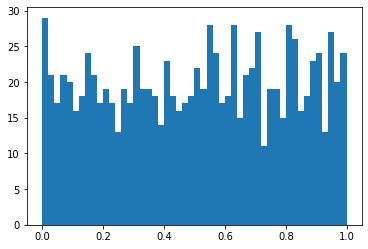
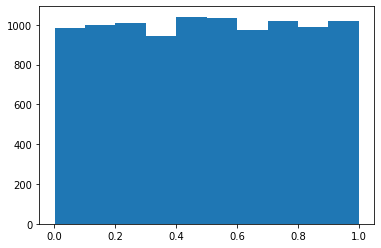
Uniform Distribution¶

A uniform distribution is a distribution in which each possible value is equally probable.

Uniform distribution on wikipedia.

from scipy.stats import uniform

data = uniform.rvs(size=10000)

plt.hist(data);

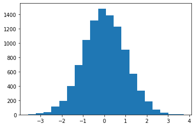
Normal Distribution¶

The Normal (also Gaussian, or 'Bell Curve') distribution, is a distribution defined by it's mean and standard deviation.

Normal distribution on wikipedia.

from scipy.stats import norm

data = norm.rvs(size=10000)

plt.hist(data, bins=20);

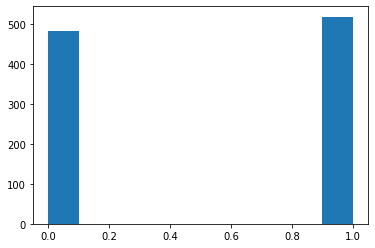
Bernouilli Distribution¶

The Bernouilli Distribution is a binary distribution - it takes only two values (0 or 1), with some probably 'p'.

Bernouilli distribution on wikipedia wikipedia.

from scipy.stats import bernoulli

data = bernoulli.rvs(0.5, size=1000)

plt.hist(data);

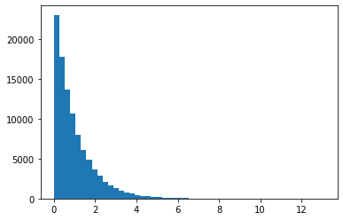
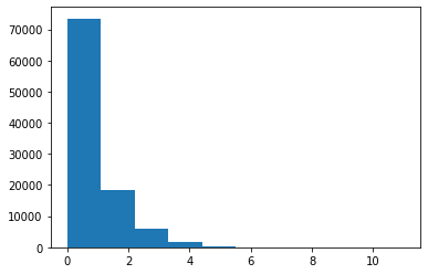
Gamma Distribution¶

The Gamma Distribution is continuous probably distribution defined by two parameters.

Gamma distribution on wikipedia.

Given different parameters, gamma distributions can look quite different. Explore different parameters.

The exponential distribution is technically a special case of the Gamma Distribution, but is also implemented separately in scipy as ‘expon’.

from scipy.stats import gamma

data = gamma.rvs(a=1, size=100000)

plt.hist(data, 50);

Beta Distribution¶

The Beta Distribution is a distribution defined on the interval [0, 1], defined by two shape parameters.

Beta distribution on wikipedia.

from scipy.stats import beta

data = beta.rvs(1, 1, size=1000)

plt.hist(data, 50);

Poisson Distribution¶

The Poisson Distribution that models events in fixed intervals of time, given a known average rate (and independent occurences).

Poisson distribution on wikipedia.

from scipy.stats import poisson

data = poisson.rvs(mu=1, size=100000)

plt.hist(data);

Data Science in Practice

Distributions

Contents